RL Training with GRPO: Kernels & Performance

30 Jan, 2026

For the last month, I’ve been living deep in the weeds of Reinforcement Learning and the bare metal. It started normally the usual ritual of staring at arxiv pdfs and watching lecture videos on a loop until the instructors sounded like frantic prophets.

But then the realization hit. Reading about an algorithm is just sightseeing. Writing the kernel? That’s the actual pilgrimage… I remembered that we have free will, so I stopped being a consumer of frameworks and started being a curator of compute.

I’ve spent the last few weeks in a haze of torch.profiler and Nvida Nsight traces, hunting down the milliseconds that the PyTorch overhead steals from us. It’s a strange kind of art, tuning the performance until the actual CUDA kernels aren't just executing, but all the threads start sounding like a high-frequency harp. We’re stripping away the bloat until all that’s left is the math and the heat of the GPU…

So, get ready to burn some GPUs and analyze the flames!!!

Blueprint :

RL and GRPO
Implementation & profiling

RL and GRPO

Reinforcement Learning (RL) has been around for over 70 years, tracing back to the early 1950s with Alan Turing’s work on pleasure-pain systems. For decades, it was confined to games and robotics, but it has now evolved into the engine behind SOTA reasoning models.

Foundation of RL algo Bellman equation:

It states that the value of your current state is the immediate reward plus the discounted value of where you land next. It’s simple recursion that forces the system to care about the future, not just the present.

$V^{π} (s) = 𝔼_{a ~ π} [R (s, a) + γ V^{π} (s^{'})]$

where,

$V^{π} (s) : Value of state s under policy π$

$R (s, a) : Immediate reward$

$γ : Discount factor$

$V^{π} (s^{'}) : Value of the next state$

The Standard: PPO

Proximal Policy Optimization (PPO) is an actor-critic RL algorithm that is standard in RL post-training of LLMs. It optimizes LLMs by maximizing the below surrogate objective:

$π_{θ} = current policy model$

$π_{θ_{o l d}} = old policy model$

$ε = clipping hyperparameter$

$A_{t} = advantage estimate$

Reward function for advantage:

$r_{ϕ} = r e w a r d m o d e l$

$π_{r e f} = r e f e r e n c e m o d e l$

$β = k l p e n a l i t y c o e f f i c i e n t$

Don’t get scared of this big math lets understand this…

The goal is simple: change the model’s weights just enough to improve performance without collapsing the policy.
Advantage is computed by applying Generalized Advantage Estimation (GAE) based on Value Function (the Critic).

PPO is powerful, but it comes with a heavy infra cost:

VRAM Hunger: The Value Function is usually a model of the same scale as the Policy. If you’re training a 70B model, you’re effectively hosting two of them.
Baseline Trap: Value Function (critic) acts as a baseline, if that itself is inaccurate, your Advantage becomes noisy.
Token-Level Overhead: Even though the final reward comes at the end of the sentence, PPO needs to estimate the every single token generated along the way.

Deepseek paper (paper link) introduced a new approach to this called GRPO:

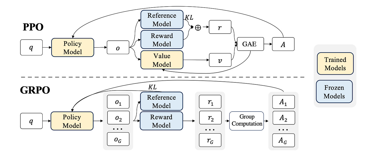
Instead of training a second model (critic) to tell us the value of a state we use average reward of multiple sampled outputs, produced in response to the same prompt, as the baseline.

GRPO

In Group Relative Policy Optimization (GRPO) for each question 𝑞, GRPO samples a group of outputs {𝑜1, 𝑜2, ….. ,𝑜𝐺} from the Old Policy. and then optimizes the model by maximizing this objective below:

$ε, β a r e h y p e r p a r a m e t e r s$

$A_{t} = a d v a n t a g e$

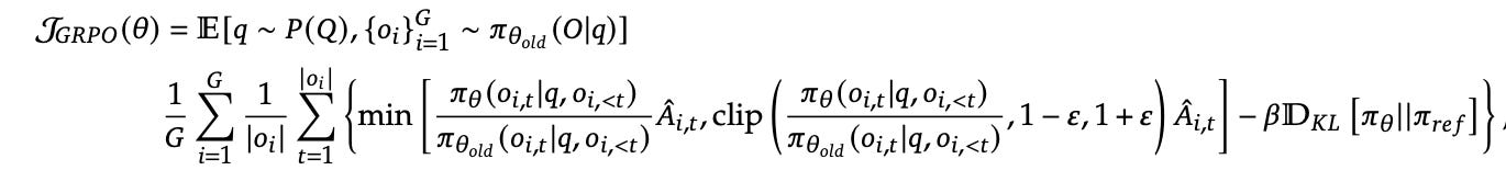
Here, advantage is calculated based on relative rewards of the outputs within the group. This is where the efficiency lies, it leverages the comparative nature of reward models without needing a critic model to guess the baseline.

To keep the model from drifting too far into the void just to chase rewards, we regularize using KL Divergence:

$(π)_{θ} = t r a i n e d p o l i c y m o d e l$

$(π)_{θ o l d} = r e f r e n c e p o l i c y m o d e l$

Pipeline Flow based on GRPO algo:

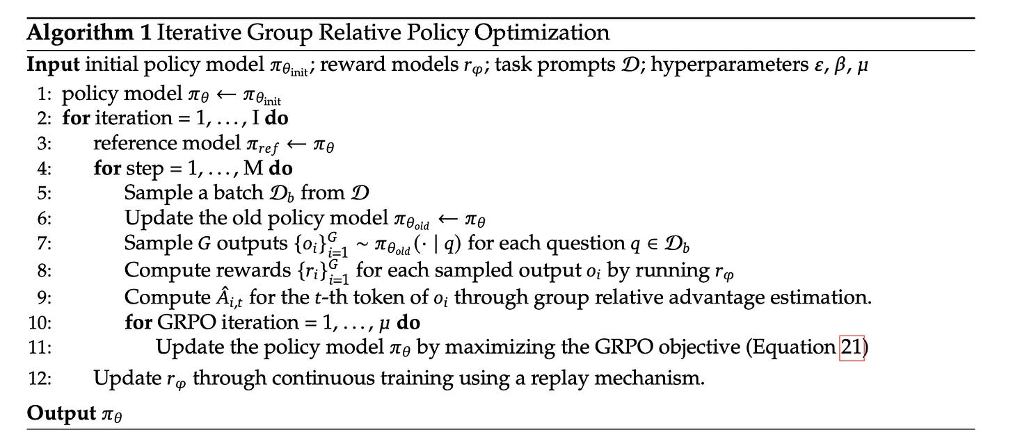
Here we assign the base model to be trained as initial policy model. This is your Current Policy. There is separate reward model that acts as judge, it assigns score based on prompt and generated output to indicate how good the response was.

For each iteration I, freeze the Current Policy and call it Reference Model. This acts as an anchor to prevent the model from drifting too far.
Then we train this combo of “frozen” reference model and “learnable” policy model for next M iteration.

We sample a batch D_b from D task prompt inputs. Current Policy is snapshotted as the Old Policy.
Now, we will generate G outputs for each q question in D_b from old policy model. Since, we have now outputs we can find the rewards for each G outputs from reward model. Then based on reward we will compute the Advantage for each token of output based on group relative advantage estimation.

Once we have generated above things, now we will apply the GRPO loop, in this we update the weights of the Current Policy, while staying close to the Reference Model by maximising the objective function and minimizing the loss.

Here, it might be confusing that what are these three policy model in equation and code.
You only need to load two versions of the model into VRAM:

The Reference Model: Frozen, used for KL calculation
The Current Policy: Learnable, this is what the optimizer updates

The Old Policy is just a snapshot of the Current Policy used for the generation phase. We don’t need a third set of weights; we just need the outputs and advantages generated before the current gradient updates began.

Implementation & profiling

The transition from theory to execution is where things usually get messy. To reach peak performance, we have to look at the code and also profile silicon.

Naive RL pipeline

grpo code:

def GRPO_step(batch):
  prompt_length = batch["plen"]
  inputs = batch["inputs"].to(model.device)
  attention_mask = batch["attention_mask"].to(model.device)
  advantages = batch["rewards"].to(model.device).unsqueeze(1) #(B,1)

  logits = model(inputs, attention_mask=attention_mask).logits[:, :-1,:]   
  input_ids = inputs[:, 1:]    # (B, L-1): 1,2,3.....l-1

  per_token_logps = get_per_token_logps(logits, input_ids)  #(B, L-1)
  per_token_logps = per_token_logps[:, prompt_length - 1: ]   

  ref_logps = batch["refs"].to(per_token_logps.device)     #(B,comp_len)

  # kl divergence
  per_token_kl = torch.exp(ref_logps - per_token_logps) - (ref_logps -         per_token_logps) - 1

  # completion mask (ignoring token)
  comp_tokens = inputs[:, prompt_length:]
  comp_mask = (comp_tokens != tokenizer.pad_token_id).float()

  # policy ratio & loss
  if "gen_logps" in batch and compute_gen_logps:
     gen_logps = batch["gen_logps"].to(model.device)
     ratio = torch.exp(per_token_logps - gen_logps)
     clipped_ratio = torch.clamp(ratio, 1 - clip_param, 1 + clip_param)
     per_token_loss = torch.min(ratio * advantages, clipped_ratio * advantages)
  else:
     # without old policy: use current logps as baseline
     per_token_loss = per_token_logps * advantages

     # final loss: -(reward - beta * kl)
     per_token_loss = -(per_token_loss - beta * per_token_kl)

     loss = (per_token_loss * comp_mask).sum(dim=1) /  (comp_mask.sum(dim=1) + 1e-8)

  return loss.mean()

To calculate the final loss, we need to reconcile three different perspectives:

The Present: We pass inputs generated by the Old Policy through the Current Policy to obtain logits and, subsequently, per_token_logps. This is what the model believes right now.
The Anchor: We retrieve ref_logps from the Reference Model, which was frozen at the start of the training iteration. Comparing these to our current logprobs allows us to calculate the KL Divergence, a sanity check that prevents the model from drifting.
The Past: We extract gen_logps (the logprobs from the old policy) and the pre-computed Advantages from our batch. These snapshots were captured before the GRPO loop began.

Once we have these three, we calculate the per_token_loss using a clipped surrogate objective. This ensures that the weight updates remain incremental and non-destructive. The final objective is framed by combining the clipped loss with the KL divergence (scaled by its beta parameter), then taking the mean over completion tokens for each group, and finally the mean over the group (G) itself.

Check the full implementation for the batch construction and the grpo_step logic here: [Link]

Profiling

v1

v1 code: [Link]

I used the NVIDIA Nsight Systems (nsys) to profile the grpo_step. To get clean, reproducible data, I fixed the max_length for prompts and generations using padding so that our profiling remains consistent, though in real production we have dynamic length input and output.

For stable performance, avoid clock throttling by locking your GPU clock speed to roughly (80–90%) of its peak clock speed.

Hardware: L4 GPU (24 GB VRAM)

gpu_env code: [Link]

The profiling logic uses NVTX to label the PyTorch operations within the nsys timeline:

def profile_grpo_step(batch):
    # warmup 
    for _ in range(5):
        optimizer.zero_grad()
        loss = GRPO_step(batch)
        loss.backward()
        optimizer.step()
    
    torch.cuda.synchronize()
    optimizer.zero_grad()
    
    # actual profile
    # emit_nvtx() connects PyTorch's record_function to Nsight Systems
    with torch.autograd.profiler.emit_nvtx():
        # Run 4 iterations as you did before
        for i in range(4):
            # nvtx.range_push/pop creates a named range visible in Nsight
            nvtx.range_push(f"Step_{i}") 
            
            # 1. Forward Pass
            with record_function("forward_pass"):
                loss = GRPO_step(batch)

            # 2. Backward Pass
            with record_function("backward_pass"):
                loss.backward()
            
            # 3. Optimizer Step
            with record_function("optimizer_step"):
                optimizer.step()
                optimizer.zero_grad()
            
            nvtx.range_pop() # End Step_i

    
    print("Profiling complete. Process exiting.")
    sys.exit(0)

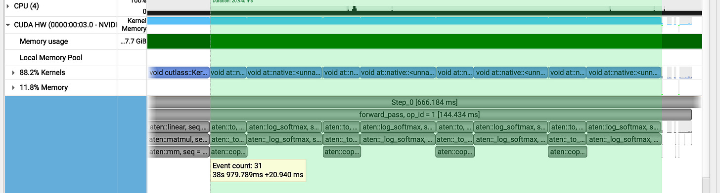
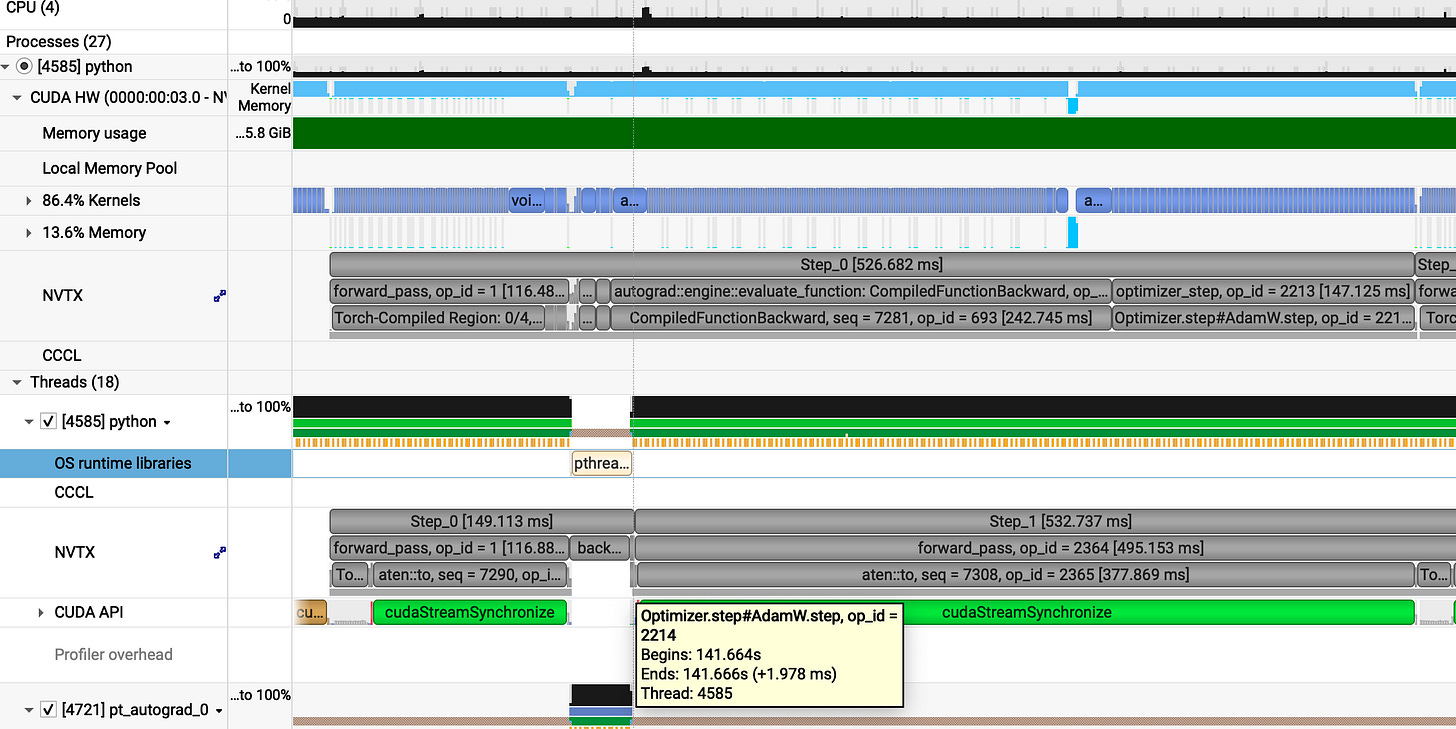
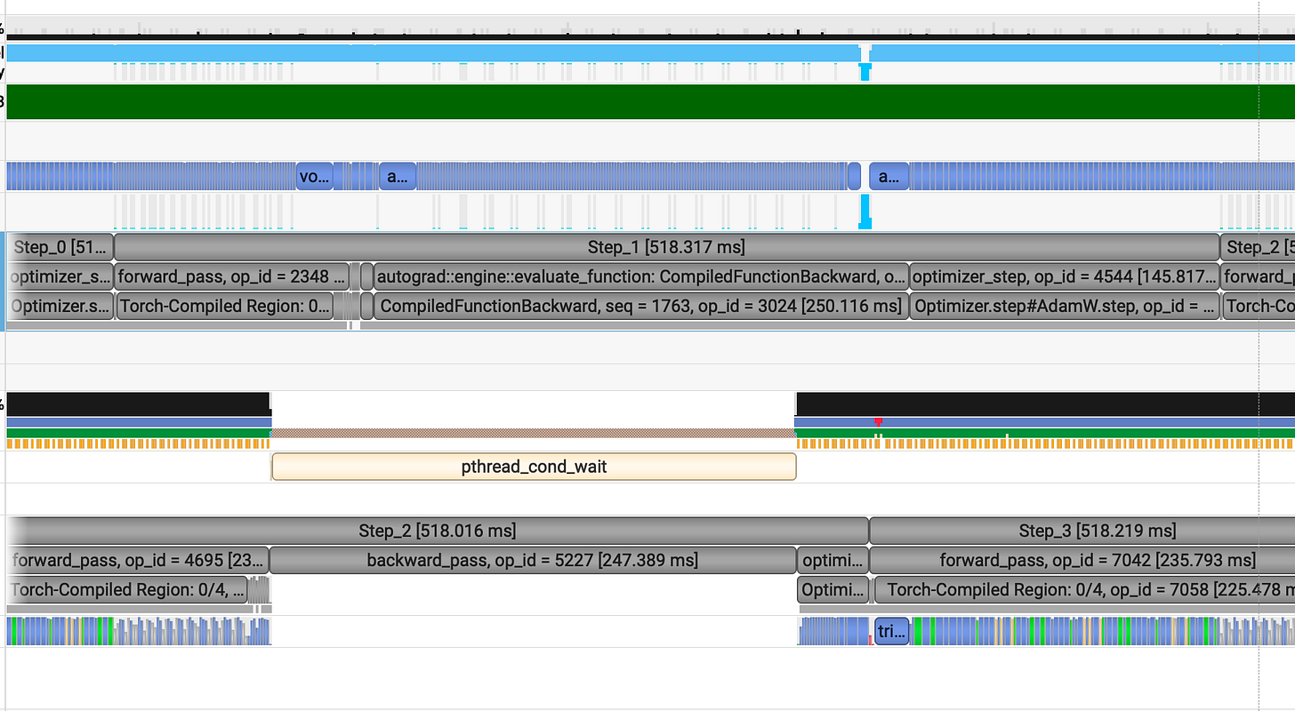
First, we perform several warmup iterations to stabilize GPU thermals and allow for any JIT overhead such as torch.compile to settle (even though it is not utilized in this naive implementation). We use NVTX alongside the PyTorch Profiler to export trace data to NVIDIA Nsight Systems (nsys). Each profiled iteration is broken down into three distinct phases: Forward Pass, Backward Pass, and Optimizer Step.

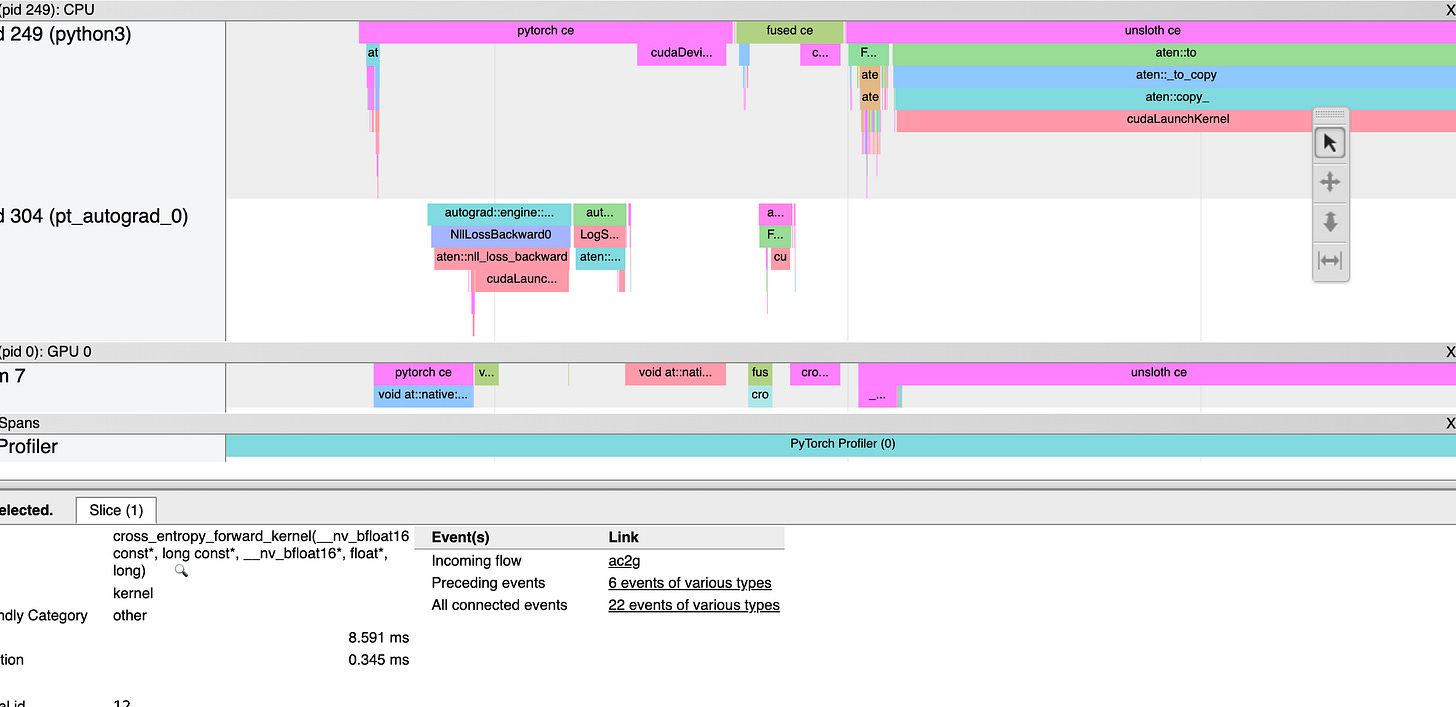
Profiling analysis:

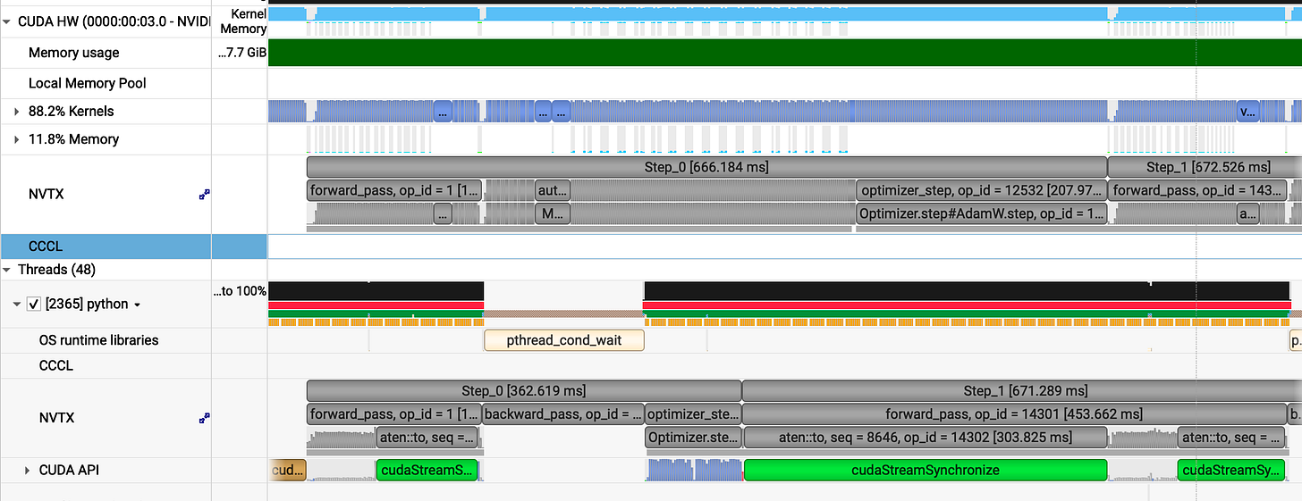
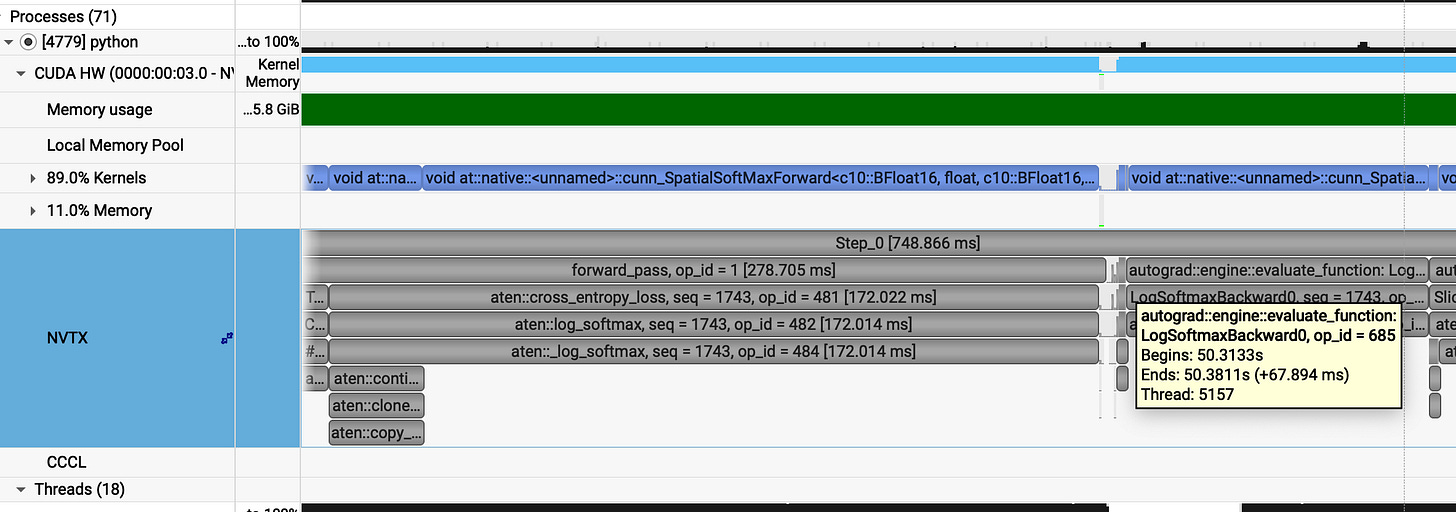
On average, each GRPO step takes 670 ms. Breaking down a single 666 ms step reveals:

Forward Pass: 144 ms
Backward Pass: 315 ms
Optimizer Step: 207 ms

The optimizer is surprisingly heavy. In GPUs, standard AdamW is memory bottlenecked by constant read/writes. Switching to a Fused AdamW will allow the GPU to load parameters into registers once, perform the math, and write them back drastically reducing HBM overhead.

Furthermore, in get_per_token_logps using a for loop with softmax + gather creates massive intermediate tensors and calculates log-probs for the entire vocab just to pick one value. We need to replace this with nn.CrossEntropyLoss or a custom fused kernel.
Finally, applying torch.compile will fuse the fragmented kernels in the forward and backward passes into lean, efficient ops.

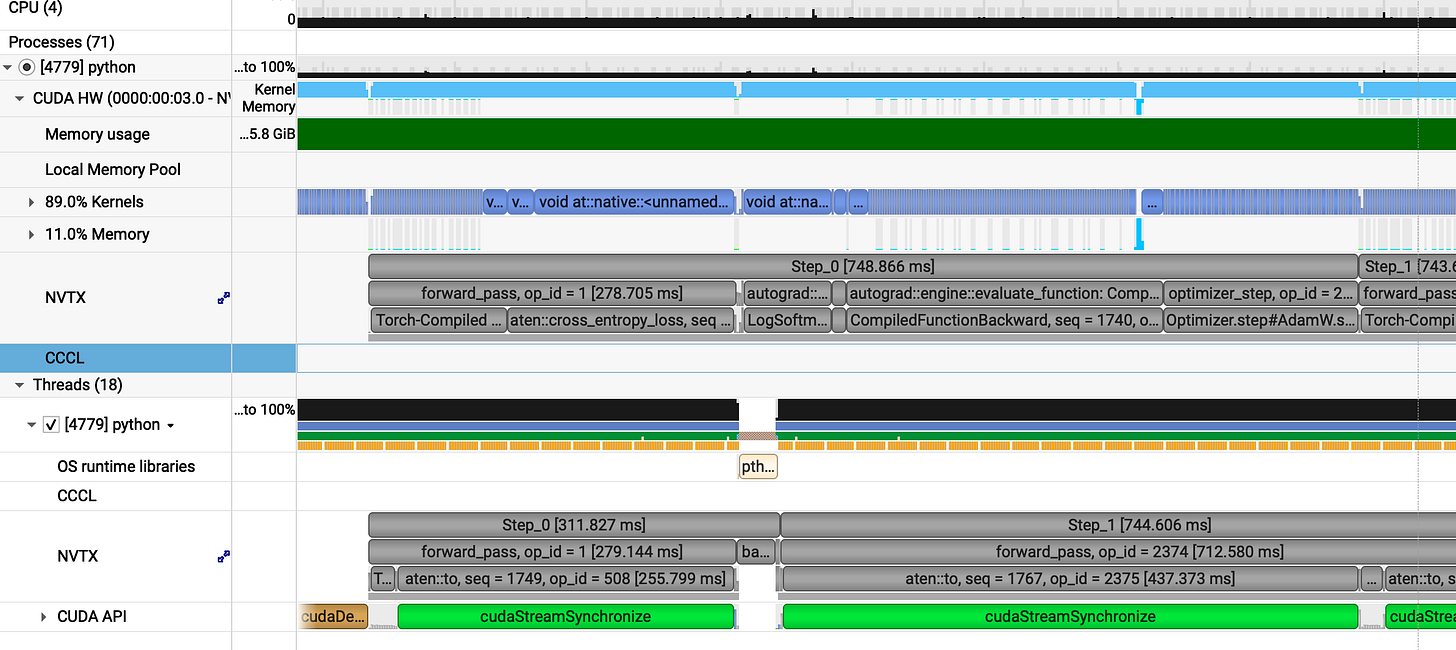
v2

v2 code : [Link]

Applied torch.compile(), switched to Fused AdamW, and replaced the manual loop with nn.CrossEntropyLoss

Profiling analysis:

Optimization isn't always so straight. Sometimes, you try to fix a leak and end up bursting a pipe :(

Average step time: 747 ms (wait, what? We went from 670 ms to 747 ms).

Now lets see any one of them (step_0 748ms):
forward_pass = 278ms
backward_pass = 322ms
optimizer_step = 148ms

The results show a significant performance gain from the fused optimizer, which now completes in 148ms compared to the previous 207ms a speedup of approximately 1.4x (40% faster). However, we observed a regression in the other phases: the forward pass increased from 144ms to 278ms, while the backward pass saw a slight, though less significant, increase from 315ms to 322ms.

Now lets catch the culprit here:

v1 (get_per_token_logps / log_softmax + gather) : forward pass) takes 20ms

v1 (get_per_token_logps / log_softmax + gather : backward pass ) takes 29ms

v2 (get_per_token_logps / cross_entropy_loss) takes 172ms for forward and 67ms for backward pass.

This abnormal behaviour can be explained by the way we applied nn.CrossEntropyLoss

# logits: [B, L, V] -> [B, V, L] for CrossEntropy
    return -nn.CrossEntropyLoss(reduction='none'(logits.transpose(1,2), input_ids)

The function expects an input shape of (N, C, d1, d2,...) where N is no. of batch and C is the class about which CE loss is calculated. To make our (B, L, V) logits compatible, we used a transpose.

In PyTorch, a transpose doesn’t actually move data in memory it just changes the strides (rule for how to access next element). Our (B, L, V) tensor is stored linearly, when we transpose it the GPU is forced to perform non-contiguous memory access to find the next element. It’s like trying to read a book but having to jump three chapters ahead for every second word.

Visualizing non_contiguous memory problem:

# (B, L-1, V): 0,1,2....l-2
logits = model(inputs, attention_mask=attention_mask).logits[:, :-1, :]   
input_ids = inputs[:, 1:]    # (B, L-1): 1,2,3.....l-1

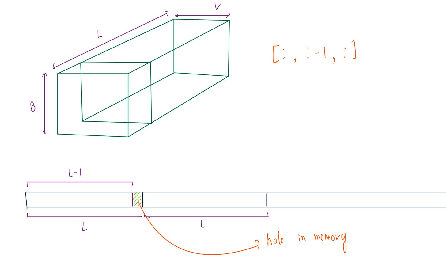
To fix this, we can’t just use .view(), because that requires the tensor to be contiguous(as our tensors are not) already. We need .reshape() which checks for contiguity and if necessary copies the data into a new, linear memory block before flattening the tensor to (B*L, V) maximising the efficiency.

def get_per_token_logps(logits, input_ids):
    # logits: [B, L, V] -> [B*L, V] for CrossEntropy
    # reshape():first check contigous then .view() on contiguous tensor
    logits_flat = logits.reshape(-1, logits.size(-1))    
    input_ids_flat = input_ids.reshape(-1)  # [B*L]
    loss_flat = -nn.CrossEntropyLoss(reduction='none')(logits_flat, input_ids_flat)
    return loss_flat.view(input_ids.shape)  # back to [B, L]

We also enabled TF32 (TensorFloat-32) a hardware feature on the L4 GPU:

# Enable TensorCores (Huge speedup for MatMul on Ampere+ GPUs)
torch.set_float32_matmul_precision('high')

FP32 consist of 32 bit: 1 bit(sign), 8 bits(exponent), 23 bits(mantissa)
TF32 consist of 19 bits: 1 bit(sign), 8 bits(exponent), 10 bits(mantissa)
TF32 keeps the 8-bit exponent of FP32 (for range) but trims the mantissa to 10 bits. The hardware performs the heavy matmuls at lightning speed and accumulates the result in FP32. We lose a bit of precision, but we gain significant throughput without sacrificing gradient stability.

v3

v3 code: [Link]

Replaced transposes with .reshape() and enabled TF32.

Profiling analysis:

AHAA!!

Average step time: ~526 ms (a massive drop from v1 670 ms and v2 747 ms)

Breaking down a single 526 ms step:
forward_pass = 116ms (down from 278 ms)
backward_pass = 263ms (down from 322 ms)
optimizer_step = 147ms (stable)

If we analyze the cross_entropy_loss part :

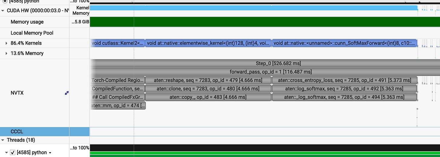
The difference is staggering. By using .reshape(), we ensured the GPU reads data linearly. The cross_entropy_loss itself now takes only 5.4 ms, though we pay a small 4.7 ms tax for the reshape operation to handle the non-contiguous slices.

The current bottleneck is that we cannot avoid the .copy() operation because our logits [B, L, V] are sliced [: , : -1, : ] making them inherently non-contiguous for any group size G (G > 1).
The next step is to bypass the native nn.CrossEntropyLoss entirely and write a customized fused CUDA kernel. This would allow us to perform the log-softmax and the loss calculation in a single pass over the memory, without intermediate copies or reshapes.

Fused cross_entropy_loss cuda kernel

To squeeze every last drop of performance we have to go below the abstraction of PyTorch. We need a Custom Fused Cross Entropy kernel.

Here is the standard formula for basic Cross-Entropy Loss:

${loss}_{i} = - \log (\frac{\exp ({logits}_{i, {label}_{i}})}{\sum_{j} \exp ({logits}_{i, j})})$

The standard approach for numeric stability is to subtract the maximum logit max_i before the exponentiation to prevent overflow:

${loss}_{i} = - \log (\frac{\exp ({logits}_{i, {label}_{i}} - {max}_{i})}{\sum_{j} \exp ({logits}_{i, j} - {max}_{i})})$

Now in pytorch and other cross entropy kernels, first we find the max_i logit by iterating through vocab size V. Then another iteration to get logsumexp_i.

${logsumexp}_{i} = {max}_{i} + \log (\sum_{j} \exp ({logits}_{i, j} - {max}_{i}))$

And then simply, calculating loss.

${loss}_{i} = {logsumexp}_{i} - x$

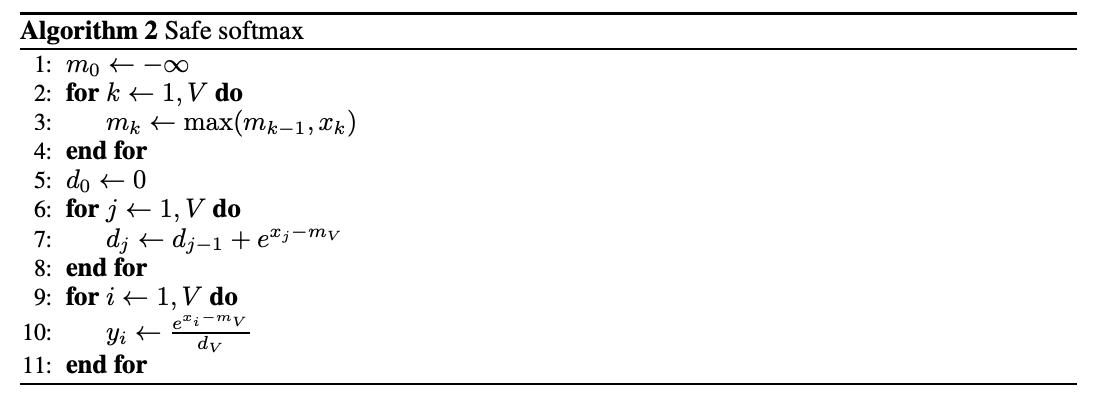
The standard approach involves a fragmented, four-step reduction.

Each thread in the block iterates through the vocabulary V to find its local maximum. These are then collapsed via warpReduce and blockReduce (using shared memory) to find the global max_i for the class.
With the global max finally known, every thread must sweep through the vocabulary again to sum the exponents: sum the exp of (logit - max) to calculate the LogSumExp.

This sum undergoes another round of warpReduce and blockReduce to produce the final logsumexp_i.
The loss is finally calculated by subtracting the target label logit from the log-sum-exp value.

By the time you finish these two full passes over the vocab, the memory bandwidth is already crying. This is why we pivot to Online Softmax to merge these passes and keep the data in the registers where it belongs.

We can collapse that fragmented process into a two-step reduction by calculating the log-sum-exp in a single pass using safe-max logic.

Each thread iterates through the vocabulary using memory coalesced loads. As it moves, it maintains a local running maximum. If a new higher logit is found, the thread updates its max and corrects the previous log-sum-exp value by adjusting the old sum to the new scale before adding the current exponent.

Once the threads finish their sweep, we use a modified warpReduce to merge these running max and sum values across the warp. We then repeat the process with a blockReduce via shared memory to synchronize the entire block.

  // local register accumulation (colaesced memory loads)
  for (int i = tid; i < logits_row_stride; i += blockDim.x) {
    float row_logit =
        __bfloat162float(row_logits[i]); 
    float m_prev = m;
    m = fmaxf(m_prev, row_logit);
	
    // branchless programming
    d = d * (__expf(m_prev - m)) + __expf(row_logit - m);
  }

I explored a branchless approach for the warp reduction to kill _thread divergence.
_Similarly i tried for warp reduction :

__device__ __forceinline__ void warp_reduce_online(float &m, float &d) {
  for (int offset = 16; offset > 0; offset /= 2) {
    float other_m = __shfl_down_sync(0xffffffff, m, offset);
    float other_d = __shfl_down_sync(0xffffffff, d, offset);

    float prev_m = m;
    m = fmaxf(m, other_m);
    d = d * (__expf(prev_m - m)) + other_d * (__expf(other_m - m));
  }
}

But in case of block reduction, you eventually have to pay the branching tax. When warp0 loads the reduced results from shared memory, only the threads within warp0 that are less than num_warp should actually do the work. The rest just sit it out so we can finalize the block’s result without junk data.

if (warp_id == 0) {
    m = (tid < num_warps) ? s_m[lane_id] : -INFINITY;
    d = (tid < num_warps) ? s_d[lane_id] : 0.0f;

    block_reduce_online(m, d);
  }

__device__ __forceinline__ void block_reduce_online(float &m, float &d) {
  for (int offset = 16; offset > 0; offset /= 2) {
    float other_m = __shfl_down_sync(0xffffffff, m, offset);
    float other_d = __shfl_down_sync(0xffffffff, d, offset);

    if (other_m > m) {
      // case: new value is larger
      d = d * __expf(m - other_m) + other_d;
      m = other_m;
    } 
    else if (other_m != -INFINITY) {
      // case: m is larger or equal, and other_m is a real number
      d += other_d * __expf(other_m - m);
    }
  }
}

I put the different reduction strategies to the test, my dual stage approach (warp_reduce_online + block_reduce_online) vs a unified warp only reduction. The latency difference was almost non-existent.

I went the branchless route to kill thread divergence. In the SIMT (Single Instruction Multiple Threads) an if/else block is a performance trap. It forces the hardware to serialize execution path by path before reconverging to execute subsequent operation.

I thought avoiding that split would help.
The reality check? The kernel is a massive memory bottleneck. The GPU spends nearly all its time pulling logits out of VRAM. Even if you reduce few cycles in the reduction logic, its just a drop in the bucket compared to the memory overhead.

fwd branchless : [Link]
fwd branched: [Link]

benchmark code : [Link]

Now, we will try to benchmark it against pytorch native nn.CrossEntropyLoss, Unsloth’s Triton cross_entropy_kernel.

Branchless warpreduce version

Branched warpreduce version

Because the performance gap was almost non existing. I stuck with the branched version. It keeps the code clean without the redundant branchless code. And the branched logic ensures __expf only called once, reducing instruction load.

Now lets compare benchmark results:
Pytorch : 1.43 ms
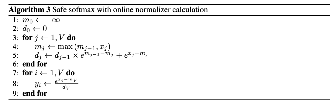
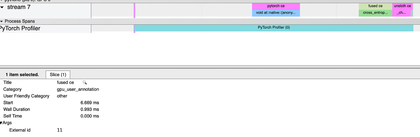
Unsloth : _0.61 ms
_Custom Fused_CE : 0.99 ms

ce fwd v2

fwd v2 code: [Link]

When we analyze our kernel the diagnosis was clear, we were drowning in memory latency. Threads spent most of the time loading logits out of VRAM one by one (though memory colaesced). To fix this I moved to vectorized loads instead of grabbing a single value, each thread pulls a massive chunk of data in one load.

// vectorized load
const float4 *vec_logits = reinterpret_cast<const float4 *>(row_logits);

int num_vectors = logits_row_stride / 8;

// local register accumulation (colaesced memory loads)
for (int i = tid; i < num_vectors; i += blockDim.x) {
	float4 vec_bits = vec_logits[i];
	// vec contains 8 bloat16 or 4 bfloat16 pairs of raw bits

	// __nv_bfloat162 cast it to seperate pair of __nv_bfloat16
	__nv_bfloat162 *pairs = reinterpret_cast<__nv_bfloat162 *>(&vec_bits);

	#pragma unroll
	for (int j = 0; j < 4; j++) {
		float2 val = __bfloat1622float2(pairs[j]);

		float m_prev = m;
		m = fmaxf(m_prev, fmaxf(val.x, val.y));

		d = d * (__expf(m_prev - m)) + __expf(val.x - m) + __expf(val.y - m);
	}
}

We used nvidia’s float4 datatype to club values together. Since our logits are in bfloat16, a single 128-bit float4 can load eight values at once. You cant just access them as (.x, .y, .z, .w) because they’re packed bits. I had to cast the float4 bits to __nv_bfloat162 pairs, then unwrap and convert them to float inside the loop for high-precision math.
One catch: float4 demands 16-byte alignment. If your data doesnt line up perfectly, the kernel crashes, so you have to write extra logic to handle the leftovers.

// leftover
int tail_start = num_vectors * 8;

// Every thread checks if there are leftovers it needs to handle
for (int i = tail_start + tid; i < logits_row_stride; i += blockDim.x) {
	__nv_bfloat16 val_bf16 = row_logits[i];
	float val = __bfloat162float(val_bf16);

	float m_prev = m;
	m = fmaxf(m_prev, val);
	d = d * (__expf(m_prev - m)) + __expf(val - m);
}

Now lets analyze perf of this version:
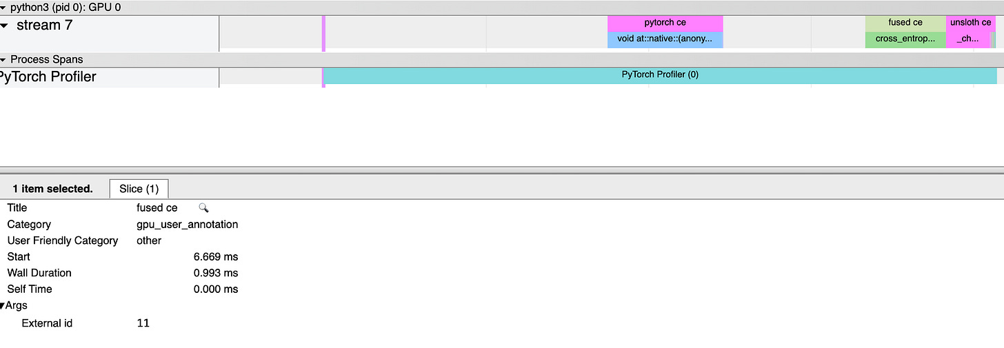
Pytorch : 1.41 ms
Unsloth : _0.61 ms
_Custom Fused_CE : 0.34 ms

wooaaah :)
By saturating the memory bus with vectorized loads, we finally beat the optimized kernels.

ce fwd v3

fwd v4 code: [Link]

For the backward pass we need the LSE (log-sum-exp) values, rather than recalculating them we simply save them during the forward pass and load them back later. Just added that part.

Backward Fused cross_entropy_loss cuda kernel

To get the model to learn we need to flow the error backward. The math behind the cross-entropy gradient is simple most of the complexity just vanishes.

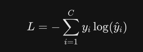
$L_{i} = - \sum_{c = 1}^{C} y_{c} \log (\frac{\exp ({logits}_{i, label_c})}{\sum_{j = 1}^{C} \exp ({logits}_{i, j})})$

Initially, we define the loss for a single sample. Since the ground truth is a one-hot encoded vector (y_c = 1 for the correct class, 0 otherwise), the total loss simplifies:

$L_{i} = - \log (\frac{\exp ({logits}_{i, target_label})}{\sum_{j = 1}^{C} \exp ({logits}_{i, j})})$

where target_label is logit in vocab where y_c = 1
We can generalize the above loss at i as L as below equation, where y_k target logprob:

$L = - \log ({\hat{y}}_{k})$

Now, we calculate the gradient of the loss with respect to the input logits:

$\frac{\partial L}{\partial l o g i t s_{i}} = \sum_{k = 1}^{C} \frac{\partial L}{\partial {\hat{y}}_{k}} \frac{\partial {\hat{y}}_{k}}{\partial l o g i t s_{i}}$

It might confuse you why we are summinng it up.
When we calculate the gradient of this loss with respect to a specific logit (x_i), we have to use the Multivariate Chain Rule. Every logit affects every softmax output, so we have to account for every path to the final loss (every y_k that is part of the loss function).

$\frac{\partial L}{\partial {\hat{y}}_{k}} = - \frac{y_{k}}{{\hat{y}}_{k}}$

Above we see how derivative of Loss w.r.t. softmax output(y_k_cap) works.
Now we will see how derivative of softmax w.r.t. logits works, here we have two cases.

First, if i = k:

$\frac{\partial {\hat{y}}_{i}}{\partial l o g i t s_{i}} = {\hat{y}}_{i} (1 - {\hat{y}}_{i})$

second if i != k:

$\frac{\partial {\hat{y}}_{k}}{\partial {logits}_{i}} = - {\hat{y}}_{k} {\hat{y}}_{i}$

Now when we combine these using the chain rule and simplify the summation, almost everything cancels out, leaving a simple formula for the gradient:

$\frac{\partial L}{\partial l o g i t s_{i}} = {\hat{y}}_{i} - y_{i}$

This implies that gradient is simply the difference between the prediction and the ground truth.
We already calculated and saved the logsumexp (lse) from the forward pass, so calculating the prediction(y_i cap) is just a quick softmax. Then, we subtract 1 if the current index is the target_label, and 0 otherwise.

${\hat{y}}_{i} = \frac{\exp ({logits}_{i})}{\sum_{j = 1}^{C} \exp ({logits}_{j})}$

Now lets write the backward cross entropy kernel

bwd v1 code: [Link]

So, here we need to handle the memory with the same aggression as the forward pass.

We load the logits using vectorized loads (float4), just like before. Each batch only needs to pull its lse (logsumexp) and target_label once. As we calculate the grad_logit, we check if the current logit index matches the target_label to substitute that 1 or 0. And finaly store in grad_logits in vectorized way.

There is one more thing which is d_loss mentioned in code it is what we call upstream gradient. This is the signal coming back from the rest of the network, telling this specific loss how much it actually contributed to the final error (just multiply our local gradient by this d_loss).

$\frac{\partial Objective}{\partial l o g i t s_{i}} = \underset{Upstream Gradient}{\underset{⏟}{\frac{\partial Objective}{\partial L}}} \times \underset{Local Gradient}{\underset{⏟}{\frac{\partial L}{\partial l o g i t s_{i}}}}$

In code,

 float grad_val1 = (__expf(val1 - logsumexp) -
                    (target_label == global_idx1 ? 1.0f : 0.0f)
                   ) * dloss;

Lets see the benchmark score:
Pytorch : 1.43 ms
Unsloth : _0.72 ms
_Custom Fused_CE : 0.82 ms

ce bwd v2

bwd v2 code : [Link]

To maximize backward pass performance, we must address the memory bottleneck caused by the massive vocabulary size (approx 156,000). At this scale, a single-block-per-row approach chokes the kernel with excessive VRAM traffic and poor SM utilization.
To solve this, we implement a 2D grid launch that breaks the vocabulary into fixed-size chunks across multiple blocks. This strategy maximizes latency hiding by ensuring all Streaming Multiprocessors (SMs) operate at max capacity.

  const int v_per_block = 2048; // 2048 vocab per block

  dim3 grid(rows, (logits_row_stride + v_per_block - 1) /
                      v_per_block); // 2048 vocab per block
  dim3 block(block_size);

Lets see the benchmark score:
Pytorch : 1.43 ms
Unsloth : _0.72 ms
_Custom Fused_CE : 0.71 ms

bwd v3 code: [Link]

We have built the engine, but to actually use it in a training loop we need to wire it into PyTorch.
We need four core files. First, cross_entropy.cu holds the actual CUDA kernels. Then we use binding.cpp to bridge the gap, it uses pybind11 (wrapped in pytorch’s PYBIND11_MODULE macro) to make our cpp/cuda functions visible to python. Here, we declare our entry points: cross_entropy_forward_launch and cross_entropy_backward_launch.

PYBIND11_MODULE(TORCH_EXTENSION_NAME, m) {
  m.def("forward", &cross_entropy_forward_launch, "Cross Entropy Forward");
  m.def("backward", &cross_entropy_backward_launch, "Cross Entropy Backward");
}

To turn this into something we can actually import we use a setup.py file which uses setuptools, and pytorch build utilities to complile our cuda/cpp code to python importable module (.so files in linux). We use CUDAExtension to tell the compiler to bundle the .cu and .cpp files, while BuildExtension handles the build with nvcc and gcc. One quick pip install . and we have a globally available fused_ce_cuda module.

Now for the high-level integration we use @torch.library.custom_op to register our kernels. This ensures they work seamlessly with torch.compile and Autograd.

We then define fused_ce_fwd and fused_ce_bwd. In the forward pass, we pre-allocate the loss and LSE tensors before invoking the custom kernel. Similarly, the backward pass takes the grad_output along with the tensors saved during the forward pass specifically the LSE, logits, and labels.
Now, @fused_ce_fwd.register_fake helps in torch.compile , when pytorch compiles a model, it performs a dry run to trace shapes and data types without actually running heavy CUDA kernels. Like if you give me a tensor of shape [B_L, V],_ I will return a loss tensor of shape [BL] and an LSE tensor of shape [B *L].
Without these, torch.compile would fail.

Finally, we wrap everything in a FusedCrossEntropy class inheriting from torch.autograd.Function (connects it to PyTorch’s Automatic Differentiation engine). The forward() pass calls the custom op and uses ctx.save_for_backward to store the logits, labels, and lse in memory. The backward() pass pulls them out and fires the backward kernel to flow the gradients.

After integrating this and applying FusedCrossEntropy() inplace of pytorch’s native nn.CrossEntropyLoss().

Lets see the benchmark results:
Pytorch forward : 1.41 ms
Pytorch backward : 1.43 ms
Unsloth forward: _0.61 ms
_Unsloth backward: _0.72 ms
_Custom Fused_CE forward : 0.35 ms
Custom Fused_CE backward : 0.71 ms

custom integrated benchmark code: [Link]

v4

v4 code: [Link]

Now, lets analyze the benchmark after integrating custom fused cross entropy.

Profiling analysis

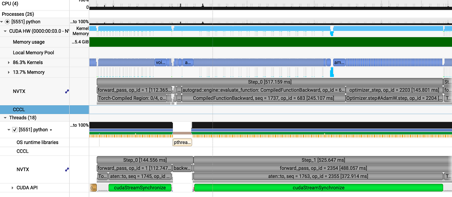
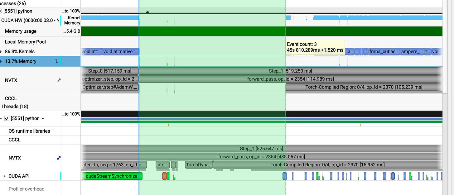
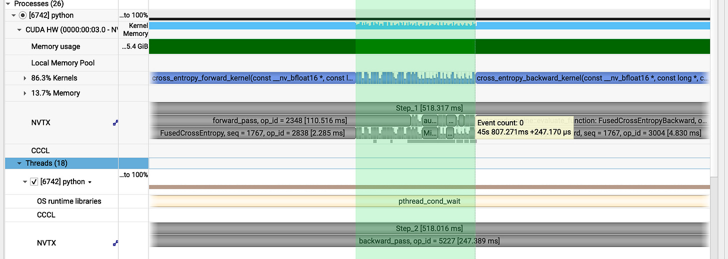
Now lets see any one of them (step_0: 518ms):
forward_pass = 113ms
backward_pass = 260ms
optimizer_step = 145ms

While we achieved a performance gain, it isn't particularly significant. Although our custom cross-entropy kernel is 2x faster than the PyTorch native implementation, it contributes very little to the overall pipeline speed.

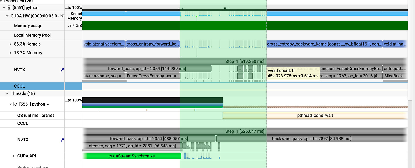
Analyzing further we can see gaps in the CUDA HW row, which indicates that the GPU is underutilized during those intervals.

When we trace these massive cudastreamSynchronize green bars :

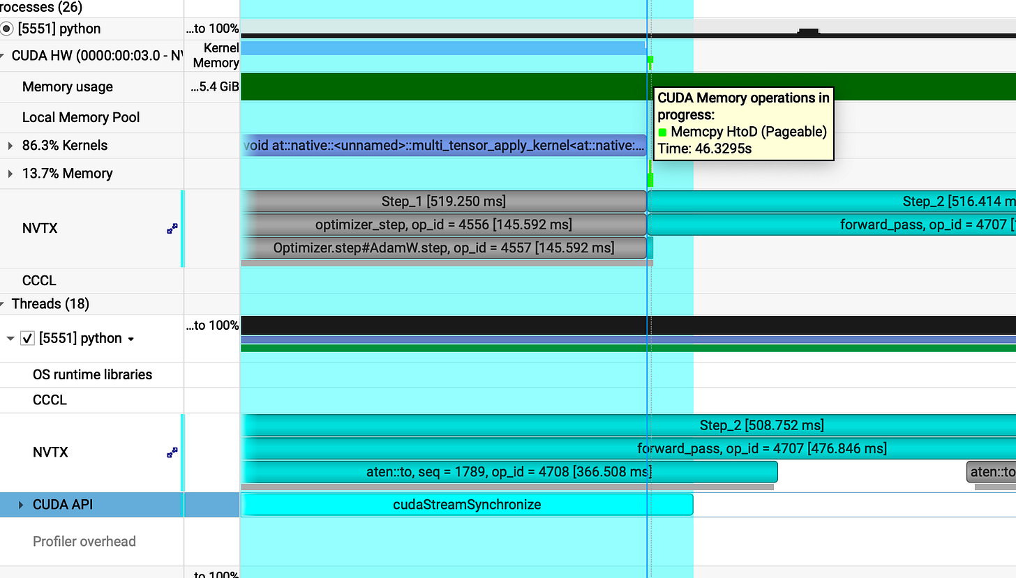
We discovered that the Memcpy operations are causing our pipeline to stall for several ms. Upon reviewing the code we identified the specific sections responsible for this behavior :

def GRPO_step(batch):
    prompt_length = batch["plen"]
    inputs = batch["inputs"].to(model.device)
    attention_mask = batch["attention_mask"].to(model.device)
    advantages = batch["rewards"].to(model.device).unsqueeze(1)   # (B, 1)

def get_ref_per_token_logps(input_ids, attention_mask, prompt_len):
    """input_ids: tokenized input,  prompt_len """
    with torch.inference_mode():
        outputs = ref_model(input_ids.to(ref_model.device), attention_mask=attention_mask.to(ref_model.device))
        logits = outputs.logits[:, :-1, :]
        shifted_ids = input_ids[:, 1:].to(ref_model.device)
        logpbs = get_per_token_logps(logits.to(torch.float32),shifted_ids)

    return logpbs[:, prompt_len - 1: ].detach().cpu()

ref_logps = batch["refs"].to(per_token_logps.device)       # (B, comp_len)

We discovered that our GRPO implementation suffers from significant H2D (Host-to-Device) latency. Currently, the batch including inputs, attention masks, advantages, and logprobs resides in pageable CPU memory. Each transfer triggers an OS overhead where pageable memory must first be staged before the actual copy occurs.

To resolve this, we can optimize our memory strategy: we will keep frequently accessed tensors such as ref_logps and gen_logps directly on the GPU across GRPO iterations. For the remaining tensors like inputs and advantages, attention_mask we will use pinned memory (page-locked). This eliminates the pageable memory overhead, ensuring that we only incur the raw memcpy cost without additional OS level bottlenecks.

in get_ref_per_token_logps:

    # detach so that no grad update flow to ref_model(just safety) as we already use torch.infernce()
    # no .cpu() off load as we have to load it again in grpo step 
    return logpbs[:, prompt_len - 1: ].detach()

during batch generation :

batch = {
        "plen": prompt_len,
        "inputs": full_ids.pin_memory(), # still in cpu in pinned memory
        "attention_mask": attention_mask.pin_memory(), # still in cpu in pinned memory
        "rewards": rewards.pin_memory(), # still in cpu in pinned memory
        "refs": ref_logps      # in gpu 
    }

We pin the memory and use non_blocking=True in the GRPO loop. This facilitates DMA(direct memory access) transfers.

v5

v5 code: [Link]

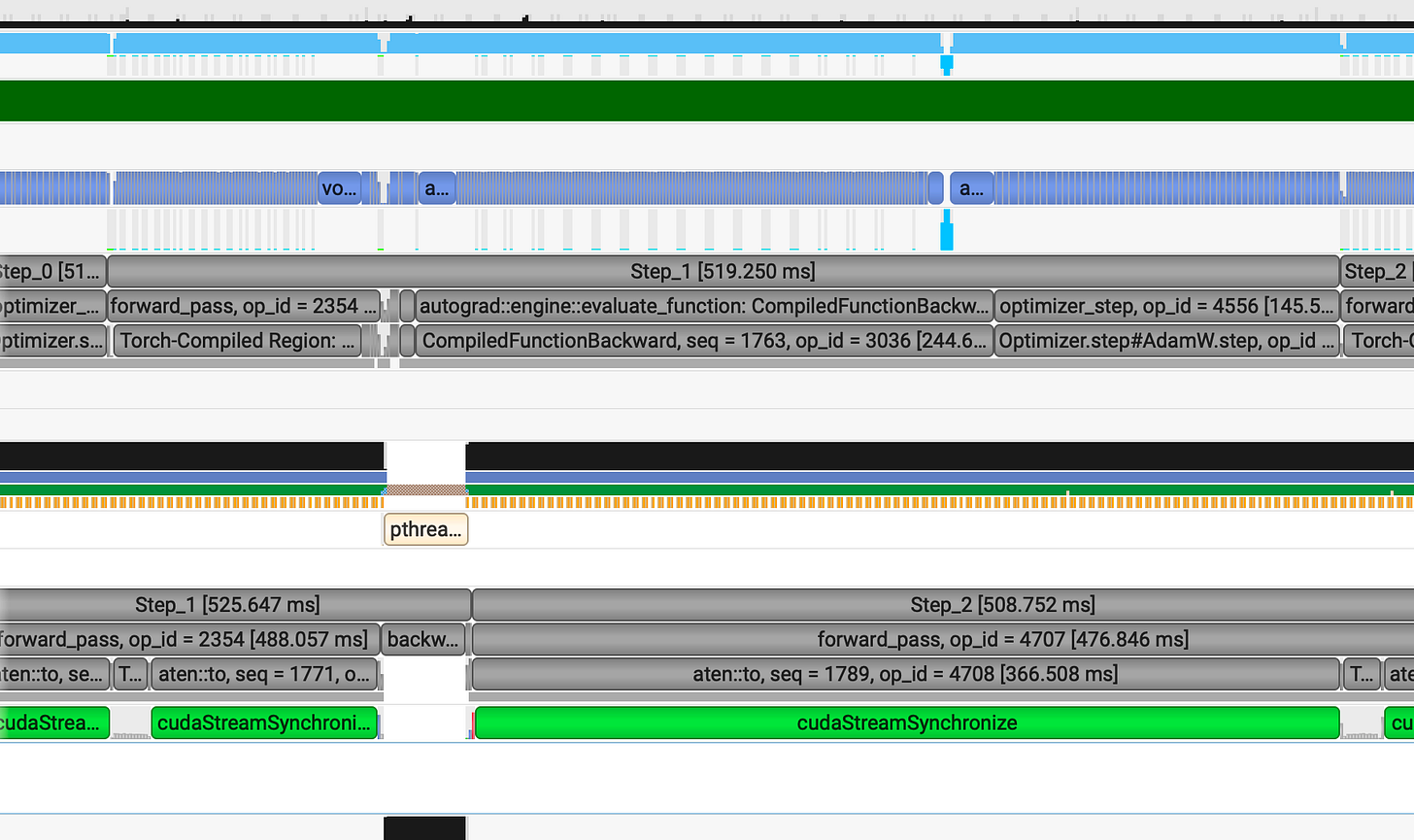
Now, lets analyze the benchmark after our pinning memory and storing tensors in gpu vram

The overall performance remains nearly identical.
However, the execution gaps previously visible in the CUDA HW trace have been eliminated.
Lets take a deeper look at why

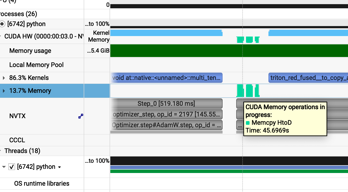
(no pageable copy)

previous gap : _1.52ms
_

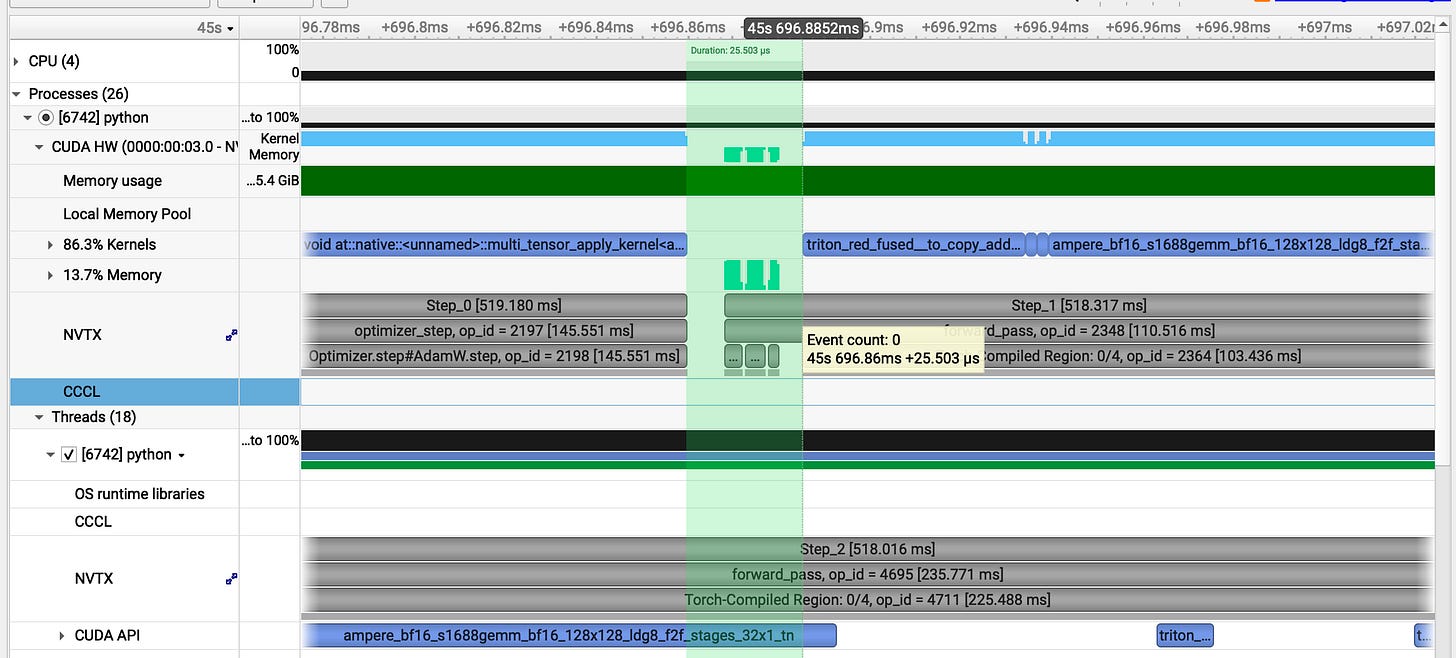
our v5 gap : **_25𝜇s

In between gap:_**

prev : 3.614ms

our v5 gap: 0.25 ms

In single step we have closed three major gaps: one at the start, one at the end and another during the execution.

When you’re training at scale, these minute gains aren’t just details they are the system. Every milisec saved is a victory against entropy.
Looking at the profiler now the result is a beautiful, continuous blue line of execution without any major breaks.

Further optimization

We could take this further by wrapping the entire GRPO_step in torch.compile, forcing the graph to fuse across the whole iteration.

Beyond that, we can leverage vLLM as a fast inference engine for the frozen ref_model for sampling phase, by offloading the generation part to a dedicated engine.

Summary

We started with a vision of Reinforcement Learning, swapping the weight of PPO for the lean logic of GRPO. We didn’t just stop at the algorithm, we went deep into the silicon profiling and benchmarking until the bottlenecks had nowhere to hide. Through customized kernels, torch.compile, and low-level memory tricks, we sculpted the system from the inside out.

I kept this journey raw to show the scars, what crashed, what lagged, and what finally soared. If there is one takeaway, its this: profile, profile, profile…
Intuition is a lie in the world of high-performance computing, the only truth is in the exec trace.

Overall, we drove the GRPO pipeline from 666ms down to ~518ms. But beyond the metrics, this was about the process the obsession with finding the art in the architecture.

Thank you for reading my piece and giving your truly valuable time :)

Code link: [Link]